Example scripts
On this page, some exemplary example scripts are presented, the scripts can be downloaded from the webpage.
Example 1 - Result import and plotting
code
# -*- coding: utf-8 -*-
"""pydoas example script 1

Introductory script illustrating how to import data from DOASIS
resultfiles. The DOASIS result file format is specified as default in the
package data file "import_info.txt".
Creates a result data set using DOASIS example data and plots some examples

"""
import pydoas
import matplotlib.pyplot as plt
from os.path import join

from SETTINGS import SAVE_DIR, SAVEFIGS, ARGPARSER, DPI, FORMAT


def main():
    plt.close("all")
    ### Get example data base path and all files in there
    _, path = pydoas.get_data_files("doasis")

    ### Device ID of the spectrometer (of secondary importance)
    dev_id = "avantes"

    ### Data import type (DOASIS result file format)
    res_type = "doasis"

    ### Specify the the import details

    # here, 3 x SO2 from the first 3 fit scenario result files (f01, f02, f03)
    # BrO from f04, 2 x O3 (f02, f04) and OClO (f04)
    import_dict = {
        'so2'  : ['SO2_Hermans_298_air_conv', ['f01','f02','f03']],
        'bro'  : ['BrO_Wil298_Air_conv', ['f04']],
        'o3'   : ['o3_221K_air_burrows_1999_conv', ['f02', 'f04']],
        'oclo' : ['OClO_293K_Bogumil_2003_conv',['f04']]}

    ### Specify the default fit scenarios for each species

    # After import, the default fit scenarios for each species are used
    # whenever fit scenarios are not explicitely specified
    default_dict = {"so2"  :   "f03",
                    "bro"  :   "f04",
                    "o3"   :   "f04",
                    "oclo" :   "f04"}

    #: Create import setup object
    stp = pydoas.dataimport.ResultImportSetup(path, result_import_dict =\
            import_dict, default_dict = default_dict, meta_import_info = res_type,\
            dev_id = dev_id)

    #: Create Dataset object for setup...
    ds = pydoas.analysis.DatasetDoasResults(stp)

    #: ... and load results
    ds.load_raw_results()

    ### plot_some_examples
    fig1, axes = plt.subplots(2, 2, figsize = (16, 8), sharex = True)
    ax = axes[0,0]

    #load all SO2 results
    so2_default = ds.get_results("so2")
    so2_fit01 = ds.get_results("so2", "f01")
    so2_fit02 = ds.get_results("so2", "f02")

    #plot all SO2 results in top left axes object
    so2_default.plot(style="-b", ax=ax, label="so2 (default, f03)")
    so2_fit01.plot(style="--c", ax=ax, label="so2 (f01)")
    so2_fit02.plot(style="--r", ax=ax, label="so2 (f02)").set_ylabel("SO2 [cm-2]")
    ax.legend(loc='best', fancybox=True, framealpha=0.5, fontsize=9)
    ax.set_title("SO2")
    fig1.tight_layout(pad = 1, w_pad = 3.5, h_pad = 3.5)

    #now load the other species and plot them into the other axes objects
    bro=ds.get_results("bro")
    bro.plot(ax=axes[0, 1], label="bro", title="BrO").set_ylabel("BrO [cm-2]")

    o3=ds.get_results("o3")
    o3.plot(ax=axes[1, 0], label="o3",
            title="O3").set_ylabel("O3 [cm-2]")
    oclo=ds.get_results("oclo")
    oclo.plot(ax=axes[1, 1], label="oclo",
              title="OClO").set_ylabel("OClO [cm-2]")

    # Now calculate Bro/SO2 ratios of the time series and plot them with
    # SO2 shaded on second y axis
    bro_so2 = bro/so2_default
    oclo_so2 = oclo/so2_default

    fig2, axis = plt.subplots(1,1, figsize=(12,8))
    bro_so2.plot(ax=axis, style=" o", label="BrO/SO2")
    oclo_so2.plot(ax=axis, style=" x", label="OClO/SO2")
    #axis.set_ylabel("BrO/SO2")
    so2_default.plot(ax=axis, kind="area",
                     secondary_y=True, alpha=0.3).set_ylabel("SO2 CD [cm-2]")
    axis.legend()
    if SAVEFIGS:
        fig1.savefig(join(SAVE_DIR, "ex1_out1.%s" %FORMAT),
                     format=FORMAT, dpi=DPI)
        fig2.savefig(join(SAVE_DIR, "ex1_out2.%s" %FORMAT),
                     format=FORMAT, dpi=DPI)

    ### IMPORTANT STUFF FINISHED (Below follow tests and display options)

    # Import script options
    options = ARGPARSER.parse_args()

    # If applicable, do some tests. This is done only if TESTMODE is active:
    # testmode can be activated globally (see SETTINGS.py) or can also be
    # activated from the command line when executing the script using the
    # option --test 1
    if int(options.test):
        ### under development
        import numpy.testing as npt
        import numpy as np
        from os.path import basename

        npt.assert_array_equal([len(so2_default),
                                ds.get_default_fit_id("so2"),
                                ds.get_default_fit_id("bro"),
                                ds.get_default_fit_id("oclo")],
                               [22, "f03", "f04", "f04"])

        vals = [so2_default.mean(),
                so2_default.std(),
                so2_fit01.mean(),
                so2_fit02.mean(),
                bro.mean(),
                oclo.mean(),
                bro_so2.mean(),
                oclo_so2.mean(),
                np.sum(ds.raw_results["f01"]["delta"])]

        npt.assert_allclose(actual=vals,
                            desired=[9.626614500000001e+17,
                                     9.785535879339162e+17,
                                     1.0835821818181818e+18,
                                     6.610916636363636e+17,
                                     126046170454545.45,
                                     42836762272727.27,
                                     0.0001389915245877655,
                                     7.579933107191676e-05,
                                     0.125067],
                            rtol=1e-7)
        print("All tests passed in script: %s" %basename(__file__))
    try:
        if int(options.show) == 1:
            plt.show()
    except:
        print("Use option --show 1 if you want the plots to be displayed")

if __name__=="__main__":
    main()
Code output
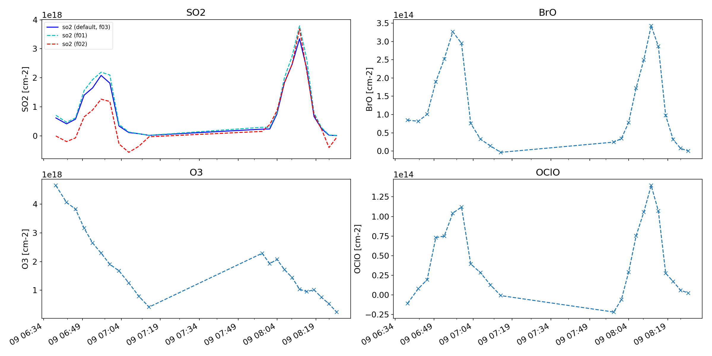
Ex1, Fig. 1: Time series of example results for 3 SO2 fits (top left), BrO (top right), O3 (bottom left) and OClO (bottom right)
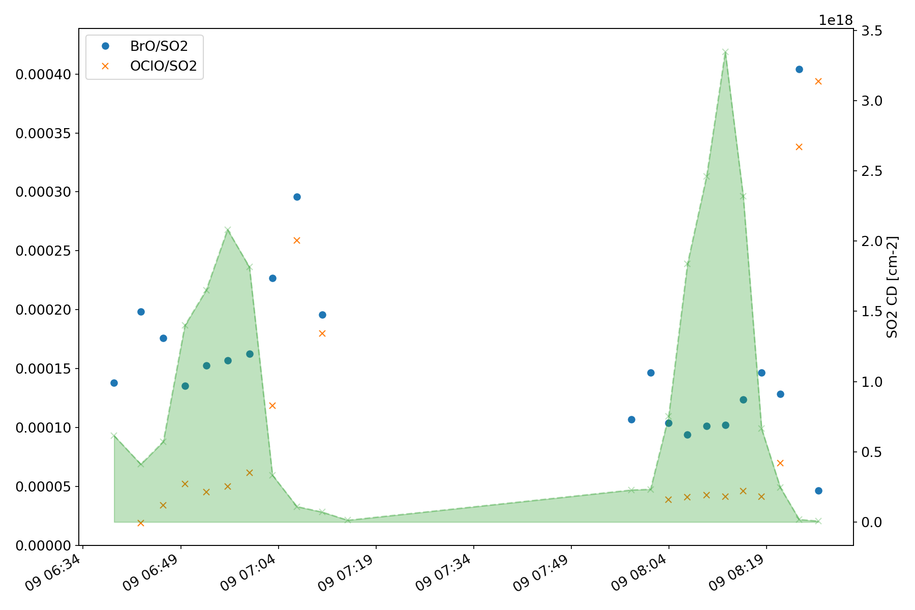
Ex2, Fig. 2: Time series of BrO/SO2 ratio (left y-axis) and corresponding SO2 CDs (green shaded, right y-axis) for same time series as shown in Fig. 1
Example 2 - Define new import type and load fake data
code
# -*- coding: utf-8 -*-
"""pydoas example script 2

In this script, a new import type is defined aiming to import the fake
data files in the package data folder "./data/fake_resultfiles
In this example, the import is performed based on specifications of the
data columns rather than based on searching the header lines of the
resultfiles.

After import, the an exemplary scatter plot of fake species 3 is performed
for the two fit IDs specified.

"""
import pydoas
from os.path import join
from collections import OrderedDict as od

from SETTINGS import SAVE_DIR, SAVEFIGS, ARGPARSER, DPI, FORMAT

def main():
    ### create some fake results:

    ### Get data path
    _, path = pydoas.inout.get_data_files(which="fake")

    ### Specify default import parameters
    # (this does not include resultfile columns of DOAS fit results)
    meta_import_info =  od([("type", "fake"),
                            ("access_type", "col_index"),
                            ("has_header_line" , 1),
                            ("time_str_formats", ["%Y%m%d%H%M"]),
                            ("file_type", "csv"),
                            ("delim", ";"),
                            ("start", 0), #col num
                            ("stop", 1), #col num
                            ("bla" , "Blub"), #invalid (for test purpose)
                            ("num_scans", 4)]) #colnum

    # You could create a new default data type now by calling
    from tempfile import NamedTemporaryFile
    with NamedTemporaryFile(mode='w+', delete=False) as temp_file:
        pydoas.inout.write_import_info_to_default_file(meta_import_info, file=temp_file.name)
    # which would add these specs to the import_info.txt file and which
    # would allow for fast access using
    # meta_info_dict = pydoas.inout.get_import_info("fake")

    import_dict = {'species1'   : [2, ['fit1']], #column 2, fit result file 1
                   'species2'   : [2, ['fit2']], #column 2, fit result file 2
                   'species3'   : [3, ['fit1', 'fit2']]} #column 3, fit result file 1 and 2

    stp = pydoas.dataimport.ResultImportSetup(path, result_import_dict =\
                import_dict, meta_import_info = meta_import_info)

    #: Create Dataset object for setup...
    ds = pydoas.analysis.DatasetDoasResults(stp)

    ax = ds.scatter_plot("species3", "fit1", "species3", "fit2",\
                    species_id_zaxis = "species1", fit_id_zaxis = "fit1")
    ax.set_title("Ex.2, scatter + regr, fake species3")

    if SAVEFIGS:
        ax.figure.savefig(join(SAVE_DIR, "ex2_out1_scatter.%s" %FORMAT),
                          format=FORMAT, dpi=DPI)

    ### IMPORTANT STUFF FINISHED (Below follow tests and display options)

    # Import script options
    options = ARGPARSER.parse_args()

    # If applicable, do some tests. This is done only if TESTMODE is active:
    # testmode can be activated globally (see SETTINGS.py) or can also be
    # activated from the command line when executing the script using the
    # option --test 1
    if int(options.test):
        import numpy.testing as npt
        from os.path import basename

        npt.assert_array_equal([],
                               [])

        # check some propoerties of the basemap (displayed in figure)

        npt.assert_allclose(actual=[],
                            desired=[],
                            rtol=1e-7)
        print("No tests implemented in script: %s" %basename(__file__))
    try:
        if int(options.show) == 1:
            from matplotlib.pyplot import show
            show()
    except:
        print("Use option --show 1 if you want the plots to be displayed")

if __name__ == "__main__":
    main()
Code output
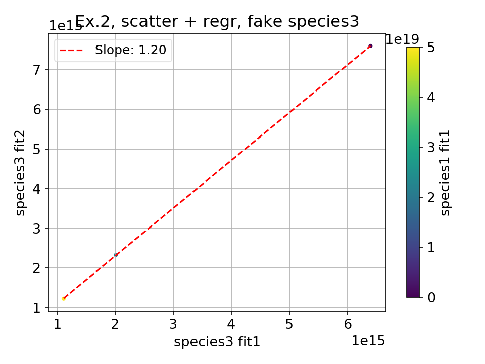
Ex2, Fig. 1: Scatter plot of fake species3 (fit1 vs. fit2) with species 1 (fit1) color coded